Introduction

In the evolving field of digital image processing, mastering histogram techniques is essential for professionals looking to enhance image quality, improve real-time processing capabilities, and effectively manage data compression and segmentation. This comprehensive guide delves deep into the application of histograms in image processing, providing working professionals with advanced strategies and detailed Python examples. From basic computation to sophisticated adaptive methods, this essay covers essential techniques that are fundamental in leveraging histograms to analyze and transform image data.

Understanding Histograms in Digital Image Processing

A histogram in digital image processing represents the frequency of pixel intensity levels across an image. This graphical tool is pivotal for various image processing tasks, such as contrast enhancement, noise reduction, and image segmentation. The histogram plots pixel intensity on the x-axis against the count of pixels with that intensity on the y-axis, providing a snapshot of the image’s contrast and brightness distribution.

Basic Histogram Computation

The first step in histogram-based image processing is computing the histogram. This involves counting the occurrence of each pixel intensity level and plotting these counts in a histogram.

"""
Python Example: Basic Histogram Computation
"""

import cv2
import numpy as np
from matplotlib import pyplot as plt

def plot_histogram(image_path):
    image = cv2.imread(image_path, cv2.IMREAD_GRAYSCALE)
    histogram = cv2.calcHist([image], [0], None, [256], [0, 256])
    plt.figure()
    plt.title("Grayscale Histogram")
    plt.xlabel("Pixel Intensity")
    plt.ylabel("Frequency")
    plt.plot(histogram)
    plt.xlim([0, 256])
    plt.show()

plot_histogram('path_to_your_image.jpg')

This script loads an image, calculates its histogram using OpenCV’s “calcHist" function, and plots it using Matplotlib. It is an essential tool for analyzing the distribution of pixel intensities in grayscale images.

Example of Histograms of images with four basic intensity characteristics

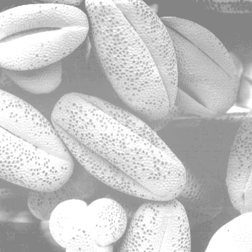
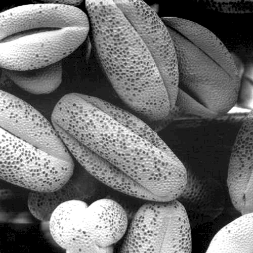
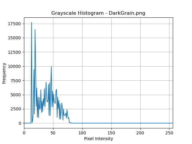
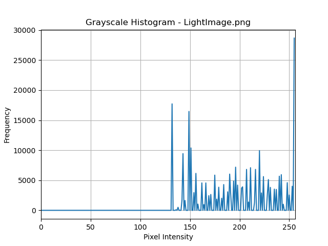
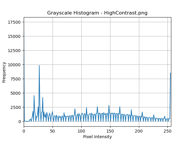
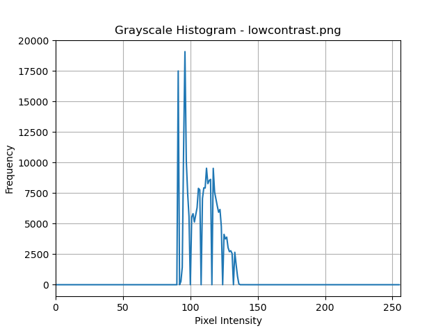
NOTE: Image Source https://www.imageprocessingplace.com/DIP-3E/dip3e_book_images_downloads.htm

Mathematical Definition of a Histogram

The histogram ‘H‘ of a digital image with gray levels in the range of [0, 𝐿−1] (where 𝐿L is the number of possible intensity levels in the image) is defined as the function:

H (𝑘) = n_𝑘​

where:

1. 𝑘 is the 𝑘^𝑡ℎ gray level.

2. n_𝑘 is the number of pixels in the image having gray level 𝑘.

3. 𝐻(𝑘) is the number of times the gray level 𝑘 occurs in the image.

For a normalized histogram, each 𝑛_𝑘 value is divided by the total number of pixels in the image (𝑁), converting it into a probability distribution:

𝑝 (𝑘) = 𝑛𝑘 / 𝑁​​

where:

1. 𝑝(𝑘) represents the probability of occurrence of the intensity level 𝑘.

2. 𝑁 is the total number of pixels in the image, 𝑁 = width × height.

Challenges and Considerations

While histogram processing is powerful, professionals must consider several challenges:

Varying Lighting Conditions: Histograms can change drastically under different lighting, which can mislead the enhancement processes.

Preservation of Natural Appearance: Over-enhancement can make images look unnatural, particularly in consumer photography where natural aesthetics are crucial.

Computational Efficiency: Processing high-resolution images requires efficient algorithms to handle the increased computational load without sacrificing performance.

Future Directions and Emerging Trends

With advancements in computational power and algorithmic design, several emerging trends are shaping the future of histogram processing:

Integration with Machine Learning: Automating histogram adjustment decisions through machine learning can optimize enhancements specific to different types of images.

Real-Time Adaptive Systems: Leveraging advanced GPUs and parallel processing technologies allows for real-time adaptive histogram adjustments in video streaming and dynamic imaging environments.

Conclusion

Histogram techniques in digital image processing offer robust tools for enhancing image quality, segmenting images, and improving real-time processing. Through detailed examples and advanced strategies provided in this guide, professionals can enhance their capability to manipulate and analyze images effectively. As the field advances, continual learning and adaptation of new histogram-based methodologies will be crucial for staying ahead in the rapidly evolving landscape of digital image processing.

This extended essay not only provides a deep dive into the practical application of histograms but also equips professionals with the knowledge to apply these techniques effectively in their work, driving forward innovations in image processing.

References

• Gonzalez, Rafael C. Digital image processing. Pearson education india, 2009.
• Burger, Wilhelm, and Mark J. Burge. Digital image processing: An algorithmic introduction. Springer Nature, 2022.
• Furht, Borko, Esad Akar, and Whitney Angelica Andrews. Digital Image Processing: Practical Approach. Springer International Publishing, 2018.
• Baskar, A., Rajappa, M., Vasudevan, S.K., & Murugesh, T.S. (2023). Digital Image Processing (1st ed.). Chapman and Hall/CRC. https://doi.org/10.1201/9781003217428.